> ## Documentation Index
> Fetch the complete documentation index at: https://anaconda.com/docs/llms.txt
> Use this file to discover all available pages before exploring further.
# Exploring project data
With Data Science & AI Workbench, you can explore project data using visualization libraries such as Bokeh and Matplotlib, and numeric libraries such as NumPy, SciPy, and Pandas.
Use these tools to discover patterns and relationships in your datasets, and develop approaches for your analysis and
deployment pipelines.
The following examples use the [Iris flower data set](https://en.wikipedia.org/wiki/Iris_flower_data_set), and this mini customer data set (`customers.csv`):
```
customer_id,title,industry
1,data scientist,retail
2,data scientist,academia
3,compiler optimizer,academia
4,data scientist,finance
5,compiler optimizer,academia
6,data scientist,academia
7,compiler optimizer,academia
8,data scientist,retail
9,compiler optimizer,finance
```
1. Begin by importing libraries, and reading data into a Pandas DataFrame:
```py theme={null}
import pandas as pd
import numpy as np
import matplotlib.pyplot as plt
irisdf = pd.read_csv('iris.csv')
customerdf = pd.read_csv('customers.csv')
%matplotlib inline
```
2. Then list column / variable names:
```py theme={null}
print(irisdf.columns)
```
```py theme={null}
Index(['sepal_length', 'sepal_width', 'petal_length', 'petal_width', 'class'], dtype='object')
```
3. Summary statistics include minimum, maximum, mean, median, percentiles, and more:
```py theme={null}
print('length:', len(irisdf)) # length of data set
print('shape:', irisdf.shape) # length and width of data set
print('size:', irisdf.size) # length * width
print('min:', irisdf['sepal_width'].min())
print('max:', irisdf['sepal_width'].max())
print('mean:', irisdf['sepal_width'].mean())
print('median:', irisdf['sepal_width'].median())
print('50th percentile:', irisdf['sepal_width'].quantile(0.5)) # 50th percentile, also known as median
print('5th percentile:', irisdf['sepal_width'].quantile(0.05))
print('10th percentile:', irisdf['sepal_width'].quantile(0.1))
print('95th percentile:', irisdf['sepal_width'].quantile(0.95))
```
```
length: 150
shape: (150, 5)
size: 750
min: 2.0
max: 4.4
mean: 3.0573333333333337
median: 3.0
50th percentile: 3.0
5th percentile: 2.3449999999999998
10th percentile: 2.5
95th percentile: 3.8
```
4. Use the `value_counts` function to show the number of items in each category, sorted
from largest to smallest. You can also set the `ascending` argument to `True` to display the list from smallest to largest.
```py theme={null}
print(customerdf['industry'].value_counts())
print()
print(customerdf['industry'].value_counts(ascending=True))
```
```
academia 5
finance 2
retail 2
Name: industry, dtype: int64
retail 2
finance 2
academia 5
Name: industry, dtype: int64
```
## Categorical variables
In statistics, a categorical variable may take on a limited number of possible
values. Examples could include blood type, nation of origin, or ratings on a
Likert scale.
Like numbers, the possible values may have an order, such as from `disagree` to `neutral` to `agree`. The values cannot, however, be used for numerical operations such as addition or division.
Categorical variables tell other Python libraries how to handle the data, so those libraries can default to suitable statistical methods or plot types.
The following example converts the `class` variable of the Iris dataset from `object` to `category`.
```py theme={null}
print(irisdf.dtypes)
print()
irisdf['class'] = irisdf['class'].astype('category')
print(irisdf.dtypes)
```
```
sepal_length float64
sepal_width float64
petal_length float64
petal_width float64
class object
dtype: object
sepal_length float64
sepal_width float64
petal_length float64
petal_width float64
class category
dtype: object
```
Within Pandas, this creates an array of the possible values, where each value appears only once, and replaces the strings in the DataFrame with indexes into the array. In some cases, this saves significant memory.
A categorical variable may have a logical order different than the lexical order. For example, for ratings on a Likert scale, the *lexical* order could alphabetize the strings and produce `agree, disagree, neither agree nor disagree, strongly agree, strongly disagree`. The *logical* order could range from most negative to most positive as `strongly disagree, disagree, neither agree nor disagree, agree, strongly agree`.
## Time series data visualization
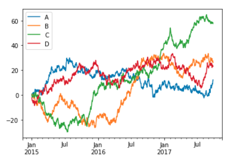
The following code sample creates four series of random numbers over time, calculates the cumulative sums for each series over time, and plots them.
```py theme={null}
timedf = pd.DataFrame(np.random.randn(1000, 4), index=pd.date_range('1/1/2015', periods=1000), columns=list('ABCD'))
timedf = timedf.cumsum()
timedf.plot()
```
 This example was adapted from [https://pandas.pydata.org/docs/user\_guide/visualization.html](https://pandas.pydata.org/docs/user_guide/visualization.html).
## Histograms
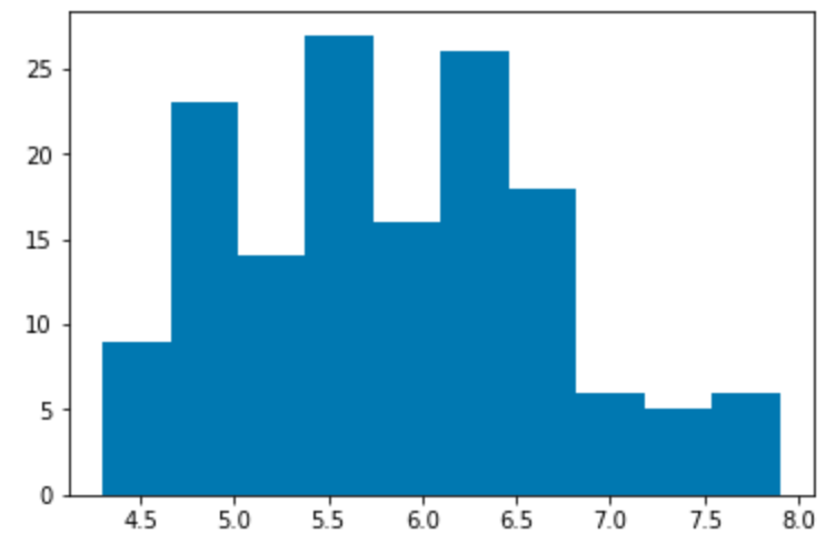
This code sample plots a histogram of the sepal length values in the Iris data set:
```py theme={null}
plt.hist(irisdf['sepal_length'])
plt.show()
```
This example was adapted from [https://pandas.pydata.org/docs/user\_guide/visualization.html](https://pandas.pydata.org/docs/user_guide/visualization.html).
## Histograms
This code sample plots a histogram of the sepal length values in the Iris data set:
```py theme={null}
plt.hist(irisdf['sepal_length'])
plt.show()
```
 ## Bar charts
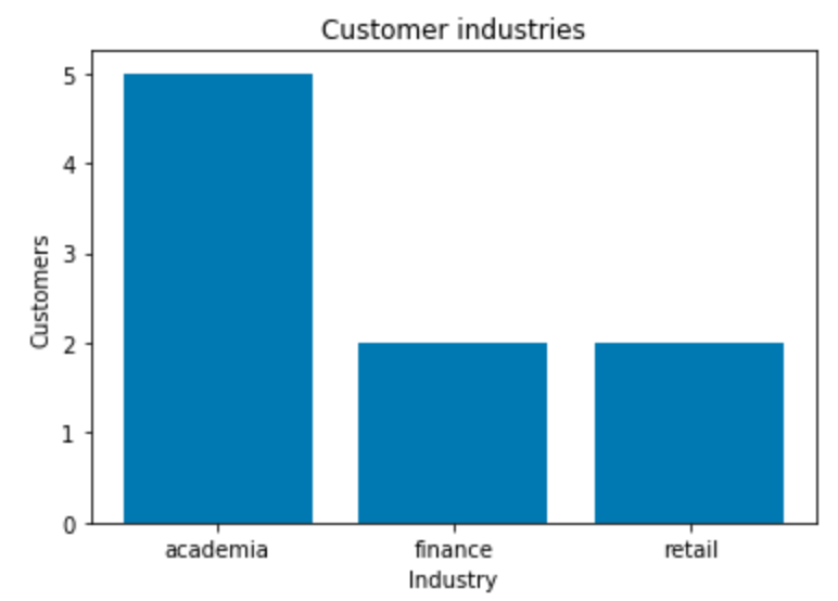
The following sample code produces a bar chart of the industries of customers in the customer
data set.
```py theme={null}
industries = customerdf['industry'].value_counts()
fig, ax = plt.subplots()
ax.bar(np.arange(len(industries)), industries)
ax.set_xlabel('Industry')
ax.set_ylabel('Customers')
ax.set_title('Customer industries')
ax.set_xticks(np.arange(len(industries)))
ax.set_xticklabels(industries.index)
plt.show()
```
## Bar charts
The following sample code produces a bar chart of the industries of customers in the customer
data set.
```py theme={null}
industries = customerdf['industry'].value_counts()
fig, ax = plt.subplots()
ax.bar(np.arange(len(industries)), industries)
ax.set_xlabel('Industry')
ax.set_ylabel('Customers')
ax.set_title('Customer industries')
ax.set_xticks(np.arange(len(industries)))
ax.set_xticklabels(industries.index)
plt.show()
```
 This example was adapted from [https://matplotlib.org/gallery/statistics/barchart\_demo](https://matplotlib.org/gallery/statistics/barchart_demo).
## Scatter plots
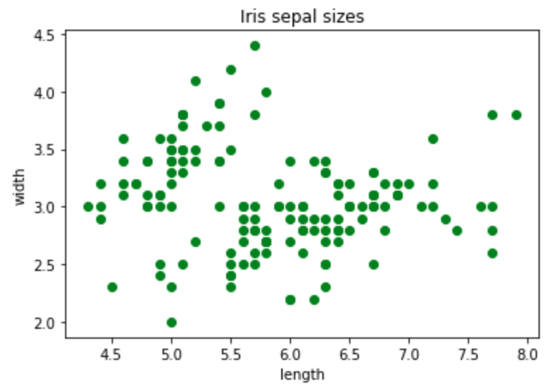
This code sample makes a scatter plot of the sepal lengths and widths in the Iris data
set:
```py theme={null}
fig, ax = plt.subplots()
ax.scatter(irisdf['sepal_length'], irisdf['sepal_width'], color='green')
ax.set(
xlabel="length",
ylabel="width",
title="Iris sepal sizes",
)
plt.show()
```
This example was adapted from [https://matplotlib.org/gallery/statistics/barchart\_demo](https://matplotlib.org/gallery/statistics/barchart_demo).
## Scatter plots
This code sample makes a scatter plot of the sepal lengths and widths in the Iris data
set:
```py theme={null}
fig, ax = plt.subplots()
ax.scatter(irisdf['sepal_length'], irisdf['sepal_width'], color='green')
ax.set(
xlabel="length",
ylabel="width",
title="Iris sepal sizes",
)
plt.show()
```
 ## Sorting
To show the customer data set:
```py theme={null}
customerdf
```
| row | customer\_id | title | industry |
| :-- | :----------- | :----------------- | :------- |
| 0 | 1 | data scientist | retail |
| 1 | 2 | data scientist | academia |
| 2 | 3 | compiler optimizer | academia |
| 3 | 4 | data scientist | finance |
| 4 | 5 | compiler optimizer | academia |
| 5 | 6 | data scientist | academia |
| 6 | 7 | compiler optimizer | academia |
| 7 | 8 | data scientist | retail |
| 8 | 9 | compiler optimizer | finance |
To sort by industry and show the results:
```py theme={null}
customerdf.sort_values(by=['industry'])
```
| row | customer\_id | title | industry |
| :-- | :----------- | :----------------- | :------- |
| 1 | 2 | data scientist | academia |
| 2 | 3 | compiler optimizer | academia |
| 4 | 5 | compiler optimizer | academia |
| 5 | 6 | data scientist | academia |
| 6 | 7 | compiler optimizer | academia |
| 3 | 4 | data scientist | finance |
| 8 | 9 | compiler optimizer | finance |
| 0 | 1 | data scientist | retail |
| 7 | 8 | data scientist | retail |
To sort by industry and then title:
```py theme={null}
customerdf.sort_values(by=['industry', 'title'])
```
| row | customer\_id | title | industry |
| :-- | :----------- | :----------------- | :------- |
| 2 | 3 | compiler optimizer | academia |
| 4 | 5 | compiler optimizer | academia |
| 6 | 7 | compiler optimizer | academia |
| 1 | 2 | data scientist | academia |
| 5 | 6 | data scientist | academia |
| 8 | 9 | compiler optimizer | finance |
| 3 | 4 | data scientist | finance |
| 0 | 1 | data scientist | retail |
| 7 | 8 | data scientist | retail |
The `sort_values` function can also use the following arguments:
* `axis` to sort either rows or columns
* `ascending` to sort in either ascending or descending order
* `inplace` to perform the sorting operation in-place, without copying the data, which can save space
* `kind` to use the quicksort, merge sort, or heapsort algorithms
* `na_position` to sort not a number (`NaN`) entries at the end or beginning
## Grouping
`customerdf.groupby('title')['customer_id'].count()` counts the items in each
group, excluding missing values such as not-a-number values (`NaN`). Because
there are no missing customer IDs, this is equivalent to
`customerdf.groupby('title').size()`.
```py theme={null}
print(customerdf.groupby('title')['customer_id'].count())
print()
print(customerdf.groupby('title').size())
print()
print(customerdf.groupby(['title', 'industry']).size())
print()
print(customerdf.groupby(['industry', 'title']).size())
```
```
title
compiler optimizer 4
data scientist 5
Name: customer_id, dtype: int64
title
compiler optimizer 4
data scientist 5
dtype: int64
title industry
compiler optimizer academia 3
finance 1
data scientist academia 2
finance 1
retail 2
dtype: int64
industry title
academia compiler optimizer 3
data scientist 2
finance compiler optimizer 1
data scientist 1
retail data scientist 2
dtype: int64
```
By default `groupby` sorts the group keys. You can use the `sort=False`
option to prevent this, which can make the grouping operation faster.
## Binning
Binning or bucketing moves continuous data into discrete chunks, which can be
used as ordinal categorical variables.
You can divide the range of the sepal length measurements into four equal bins:
```py theme={null}
pd.cut(irisdf['sepal_length'], 4).head()
```
```
0 (4.296, 5.2]
1 (4.296, 5.2]
2 (4.296, 5.2]
3 (4.296, 5.2]
4 (4.296, 5.2]
Name: sepal_length, dtype: category
Categories (4, interval[float64]): [(4.296, 5.2] < (5.2, 6.1] < (6.1, 7.0] < (7.0, 7.9]]
```
Or make a custom bin array to divide the sepal length measurements into
integer-sized bins from 4 through 8:
```py theme={null}
custom_bin_array = np.linspace(4, 8, 5)
custom_bin_array
```
```py theme={null}
array([4., 5., 6., 7., 8.])
```
Copy the Iris data set, and apply the binning to it:
```py theme={null}
iris2=irisdf.copy()
iris2['sepal_length'] = pd.cut(iris2['sepal_length'], custom_bin_array)
iris2['sepal_length'].head()
```
```
0 (5.0, 6.0]
1 (4.0, 5.0]
2 (4.0, 5.0]
3 (4.0, 5.0]
4 (4.0, 5.0]
Name: sepal_length, dtype: category
Categories (4, interval[float64]): [(4.0, 5.0] < (5.0, 6.0] < (6.0, 7.0] < (7.0, 8.0]]
```
Then plot the binned data:
```py theme={null}
plt.style.use('ggplot')
categories = iris2['sepal_length'].cat.categories
ind = np.array([x for x, _ in enumerate(categories)])
plt.bar(ind, iris2.groupby('sepal_length').size(), width=0.5, label='Sepal length')
plt.xticks(ind, categories)
plt.show()
```
## Sorting
To show the customer data set:
```py theme={null}
customerdf
```
| row | customer\_id | title | industry |
| :-- | :----------- | :----------------- | :------- |
| 0 | 1 | data scientist | retail |
| 1 | 2 | data scientist | academia |
| 2 | 3 | compiler optimizer | academia |
| 3 | 4 | data scientist | finance |
| 4 | 5 | compiler optimizer | academia |
| 5 | 6 | data scientist | academia |
| 6 | 7 | compiler optimizer | academia |
| 7 | 8 | data scientist | retail |
| 8 | 9 | compiler optimizer | finance |
To sort by industry and show the results:
```py theme={null}
customerdf.sort_values(by=['industry'])
```
| row | customer\_id | title | industry |
| :-- | :----------- | :----------------- | :------- |
| 1 | 2 | data scientist | academia |
| 2 | 3 | compiler optimizer | academia |
| 4 | 5 | compiler optimizer | academia |
| 5 | 6 | data scientist | academia |
| 6 | 7 | compiler optimizer | academia |
| 3 | 4 | data scientist | finance |
| 8 | 9 | compiler optimizer | finance |
| 0 | 1 | data scientist | retail |
| 7 | 8 | data scientist | retail |
To sort by industry and then title:
```py theme={null}
customerdf.sort_values(by=['industry', 'title'])
```
| row | customer\_id | title | industry |
| :-- | :----------- | :----------------- | :------- |
| 2 | 3 | compiler optimizer | academia |
| 4 | 5 | compiler optimizer | academia |
| 6 | 7 | compiler optimizer | academia |
| 1 | 2 | data scientist | academia |
| 5 | 6 | data scientist | academia |
| 8 | 9 | compiler optimizer | finance |
| 3 | 4 | data scientist | finance |
| 0 | 1 | data scientist | retail |
| 7 | 8 | data scientist | retail |
The `sort_values` function can also use the following arguments:
* `axis` to sort either rows or columns
* `ascending` to sort in either ascending or descending order
* `inplace` to perform the sorting operation in-place, without copying the data, which can save space
* `kind` to use the quicksort, merge sort, or heapsort algorithms
* `na_position` to sort not a number (`NaN`) entries at the end or beginning
## Grouping
`customerdf.groupby('title')['customer_id'].count()` counts the items in each
group, excluding missing values such as not-a-number values (`NaN`). Because
there are no missing customer IDs, this is equivalent to
`customerdf.groupby('title').size()`.
```py theme={null}
print(customerdf.groupby('title')['customer_id'].count())
print()
print(customerdf.groupby('title').size())
print()
print(customerdf.groupby(['title', 'industry']).size())
print()
print(customerdf.groupby(['industry', 'title']).size())
```
```
title
compiler optimizer 4
data scientist 5
Name: customer_id, dtype: int64
title
compiler optimizer 4
data scientist 5
dtype: int64
title industry
compiler optimizer academia 3
finance 1
data scientist academia 2
finance 1
retail 2
dtype: int64
industry title
academia compiler optimizer 3
data scientist 2
finance compiler optimizer 1
data scientist 1
retail data scientist 2
dtype: int64
```
By default `groupby` sorts the group keys. You can use the `sort=False`
option to prevent this, which can make the grouping operation faster.
## Binning
Binning or bucketing moves continuous data into discrete chunks, which can be
used as ordinal categorical variables.
You can divide the range of the sepal length measurements into four equal bins:
```py theme={null}
pd.cut(irisdf['sepal_length'], 4).head()
```
```
0 (4.296, 5.2]
1 (4.296, 5.2]
2 (4.296, 5.2]
3 (4.296, 5.2]
4 (4.296, 5.2]
Name: sepal_length, dtype: category
Categories (4, interval[float64]): [(4.296, 5.2] < (5.2, 6.1] < (6.1, 7.0] < (7.0, 7.9]]
```
Or make a custom bin array to divide the sepal length measurements into
integer-sized bins from 4 through 8:
```py theme={null}
custom_bin_array = np.linspace(4, 8, 5)
custom_bin_array
```
```py theme={null}
array([4., 5., 6., 7., 8.])
```
Copy the Iris data set, and apply the binning to it:
```py theme={null}
iris2=irisdf.copy()
iris2['sepal_length'] = pd.cut(iris2['sepal_length'], custom_bin_array)
iris2['sepal_length'].head()
```
```
0 (5.0, 6.0]
1 (4.0, 5.0]
2 (4.0, 5.0]
3 (4.0, 5.0]
4 (4.0, 5.0]
Name: sepal_length, dtype: category
Categories (4, interval[float64]): [(4.0, 5.0] < (5.0, 6.0] < (6.0, 7.0] < (7.0, 8.0]]
```
Then plot the binned data:
```py theme={null}
plt.style.use('ggplot')
categories = iris2['sepal_length'].cat.categories
ind = np.array([x for x, _ in enumerate(categories)])
plt.bar(ind, iris2.groupby('sepal_length').size(), width=0.5, label='Sepal length')
plt.xticks(ind, categories)
plt.show()
```
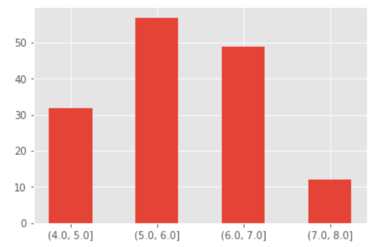 This example was adapted from [http://benalexkeen.com/bucketing-continuous-variables-in-pandas/](http://benalexkeen.com/bucketing-continuous-variables-in-pandas/).